How To Use HAPPy:

• Download this page as a Python code file;

• Download this page as a Jupyter notebook (no outputs);

• Download this page as a Jupyter notebook (with outputs).

Import packages

Hint

If running in the IPython console, consider running %matplotlib to enable interactive plots. If running in the Jupyter Notebook, use %matplotlib inline.

>>> # First import matplotlib (for plotting) and skan
>>> from matplotlib import pyplot as plt
>>> from skan import draw
>>> import numpy as np
>>> from skimage import exposure
>>>
>>> # Then import the radial hydride packagess
>>> from HAPPY import import_image
>>> from HAPPY import cropping_functions as crop
>>> from HAPPY import plot_functions as plt_f
>>> from HAPPY import radial_hydride_fraction as RHF
>>> from HAPPY import branching as branch
>>> from HAPPY import crack_path as cp
>>> from HAPPY import image_processing

Importing Image

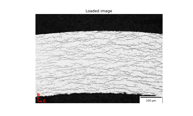
• First, import the image using the import_image command. Transpose the image if necessary using the transpose argument to make the radial direction vertical.

• The cropImage function applies a rectangular crop to the image to remove scale bars, or if you have a specific rectangular region you want to look at.

• Input Scale Bar Value in Scale_Bar_Micron_Value and Pixels_In_Scale_Bar, the scale bar will then be calculated.

>>> # Load image
>>> original_image = import_image.image(image_path ='data/520-5b.png', transpose = False)
>>> cropped_image = crop.cropImage(original_image, crop_bottom=50, crop_top=0, crop_left=0, crop_right=0)
>>> crop1 = cropped_image
>>> # Input the value of the scale bar in microns
>>> Scale_Bar_Micron_Value = 100
>>> #Input how many pixels are in your scale bar
>>> Pixels_In_Scale_Bar = 165.5
>>> Scale_Bar_Value_In_Meters = Scale_Bar_Micron_Value*(1e-6)
>>> scale = Scale_Bar_Value_In_Meters/Pixels_In_Scale_Bar
>>> scale_um = scale*1e6
>>> location = 'lower right'
>>>
>>>
>>> # Plot image
>>> plt_f.plot(img=cropped_image, title='Loaded image',scale=scale, location=location)

(png, hires.png, pdf)

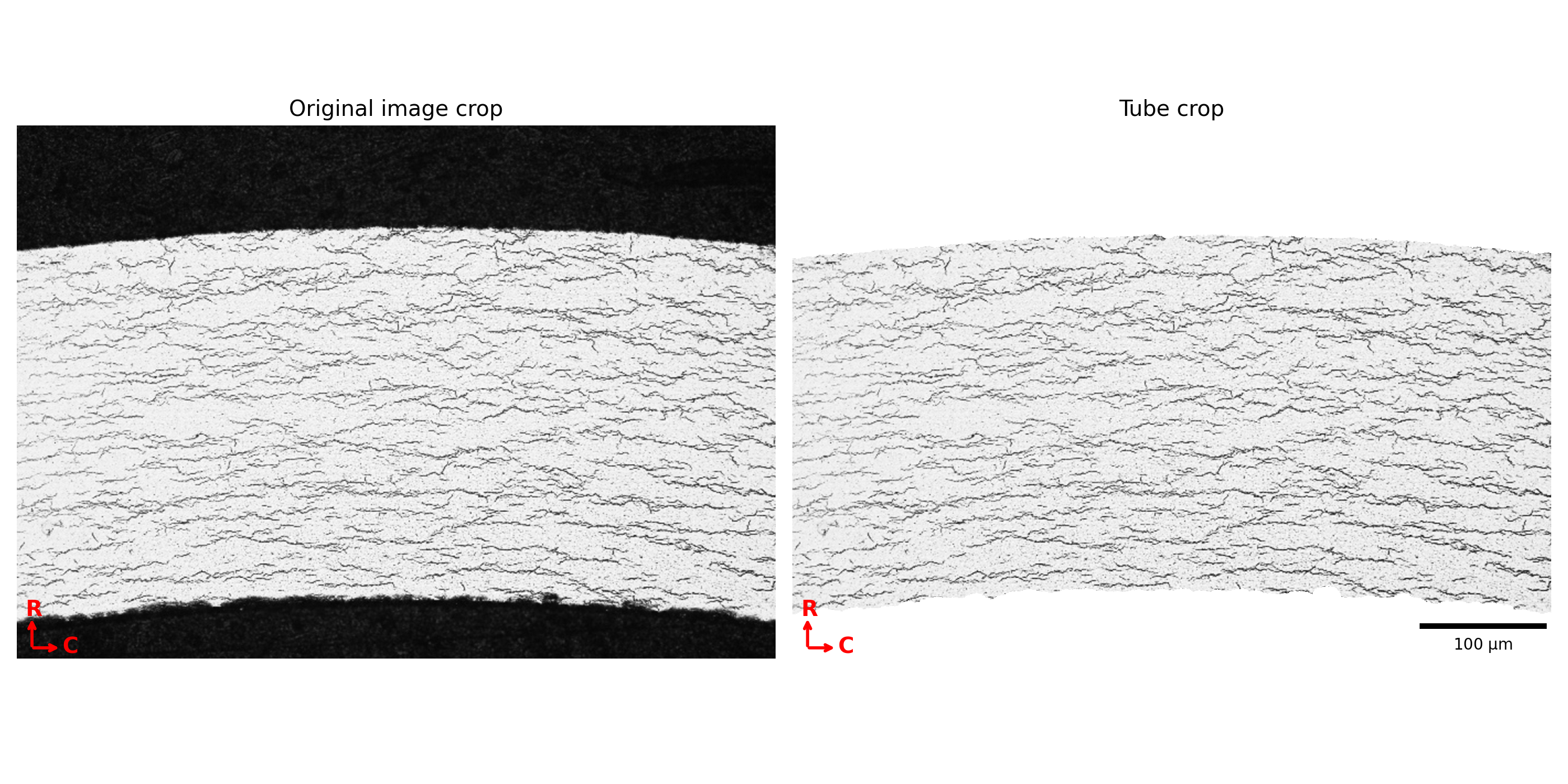
Additional Cropping

The second crop function is cropping_tube, which should be used if the micrograph is curved and removes black pats of the image which are not the tube. A crop_param of around 0.1-0.2 is reccomended.

>>> # Crop tube
>>> cropped_image, crop_threshold = crop.cropping_tube(cropped_image,
...                                                    crop_param = 0.2, size_param = 1000, dilation_param = 10)
...
>>> # Plot comparison
>>> plt_f.plot_comparison(crop1, 'Original image crop', cropped_image, 'Tube crop',scale=scale,
...                    location=location)

(png, hires.png, pdf)

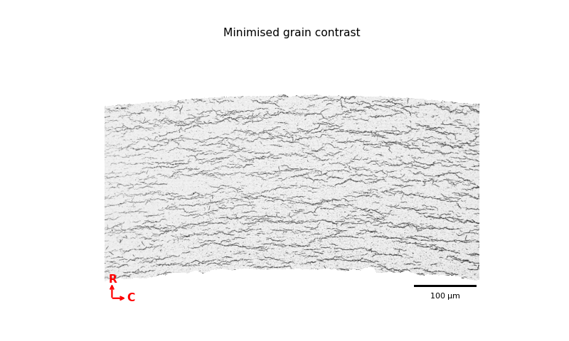
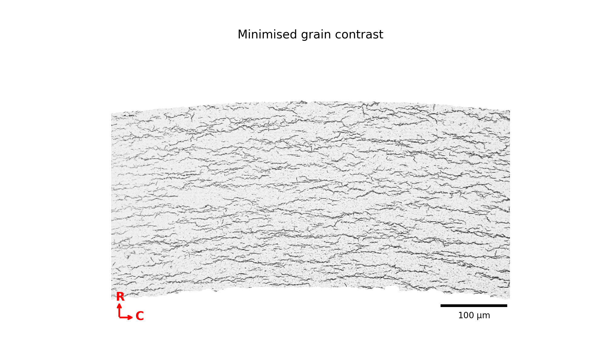
Image Processing

Grain contast or uneven lighting can be minimised through the application of a gaussian blur in the minimize_grain_contrast function. A value of 10 seems to work for most cases.

>>> # Remove grain contrast
>>> removed_grains = image_processing.minimize_grain_contrast(cropped_image, sigma = 10)
>>>
>>> # Plot image
>>> plt_f.plot(img=cropped_image, title='Minimised grain contrast', scale=scale, location=location)
>>>
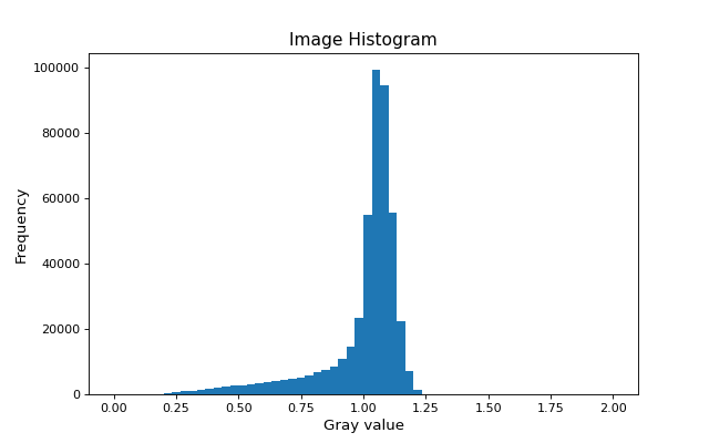
>>> # Plot the histogram for removed grains so that we can see where we should threshold
>>> histogram = plt_f.plot_hist(removed_grains)
>>>
>>> # Print an approximate threshold value which should work well
>>> print('Approximate threshold: {0:.3f}'.format(
...     2*np.nanmedian(removed_grains)-np.nanpercentile(removed_grains, 90)))

(png, hires.png, pdf)

(png, hires.png, pdf)

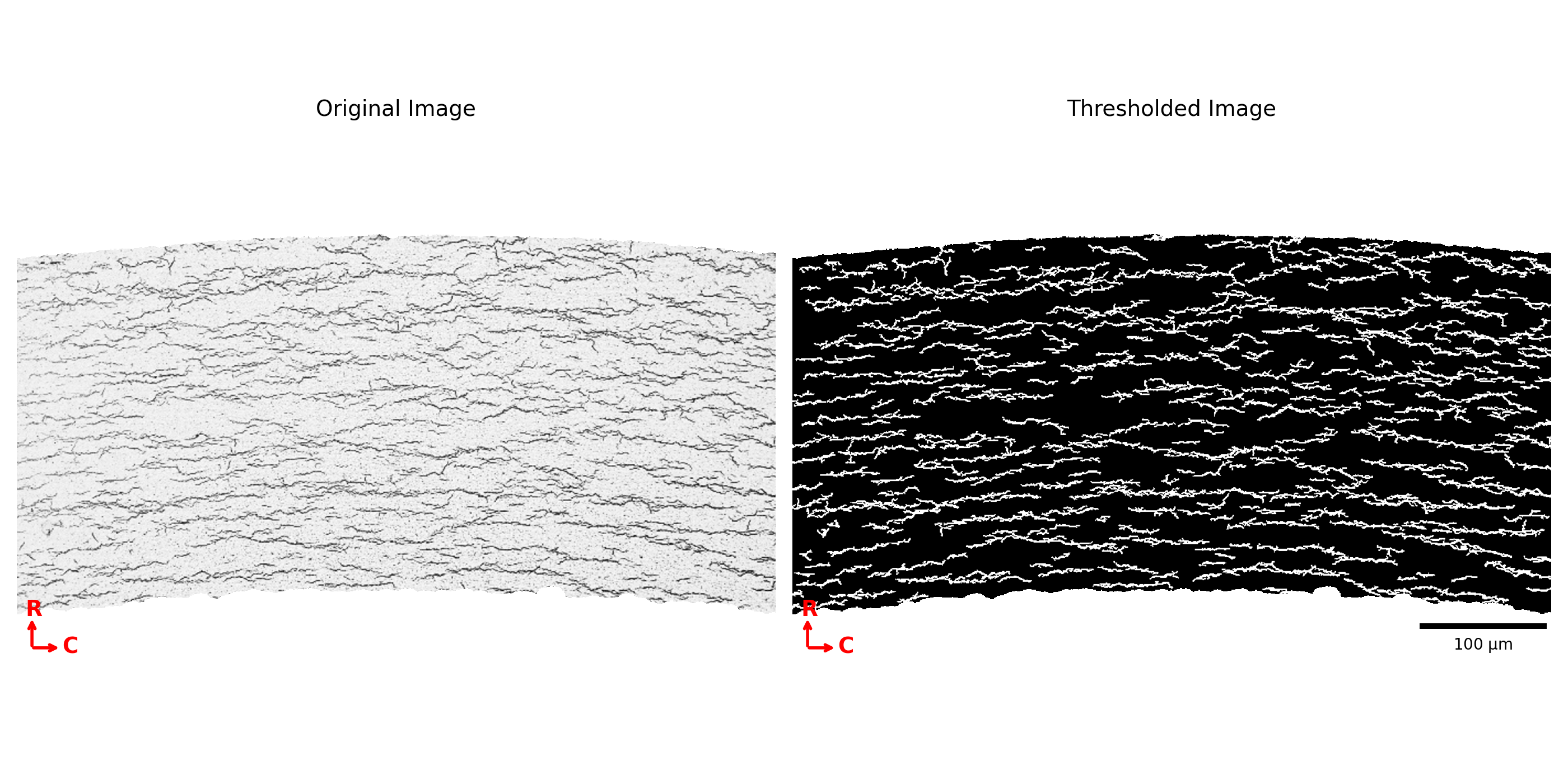
Thresholding

After this, the image is thresholded using the simple_threshold function. The threshold value should be set using the threshold argument. Small features, less than a given size in microns small_obj can optionally be removed. Note it is important not too over threshold the image, guidance of a value to threshold is shown above and can be determined by investigating the histograms plotted above.

>>> # Apply threshold
>>> thres = image_processing.simple_threshold(removed_grains,scale_um, crop_threshold,
...                                           threshold = 0.98, small_obj = 40)
...
>>> # Plot the thresholded image and compare it to the original image:
>>> plt_f.plot_comparison(cropped_image, 'Original Image', thres,'Thresholded Image', scale=scale,location=location)

(png, hires.png, pdf)

The first step is to perform the hough line transform hough_rad there are a few input parameters that should be considered: - num_peaks: should be changed dependent on the type of micrograph, if your hydrides are straight and not very interconnected a small value of around 2 is good, if in one box, there are many branches that need to be picked up, this value should be increased accordingly to a value of 5 or more. - min_dist, min_angle and val are pre-set and seem to work for most cases.

>>> # Apply Hough transform
>>> angle_list,len_list = RHF.hough_rad(thres, num_peaks=2, scale=scale, location=location)

(png, hires.png, pdf)

>>> #Non weighted radial hydride fraction
>>> radial, circumferential = RHF.RHF_no_weighting_factor(angle_list, len_list)
>>>
>>> print('The non-weighted RHF  is {0:.4f}'.format(radial))

>>> #Weighted Radial Hydride Fraction
>>> fraction = RHF.weighted_RHF_calculation(angle_list, len_list)
>>>
>>> print('The weighted RHF is: {0:.4f}'.format(fraction))

Other Methods for Radial Hydride Fraction Calculation

Here all four different RHF calculation methods are shown in the graph

>>> #chu radial hydride calculation
>>> deg_angle_list = np.rad2deg(angle_list)
>>>
>>> radial_list_chu=[]
>>> circum_list_chu = []
>>>
>>> for k in deg_angle_list:
...     if (k>0 and k<40) or (k>-40 and k<0) :
...         radial_list_chu.append(len_list)
...     elif (k>50 and k<90) or (k>-90 and k<-50):
...         circum_list_chu.append(len_list)
...
...
>>> rad_hyd_chu = np.sum(radial_list_chu)
>>> cir_hyd_chu = np.sum(circum_list_chu)
>>>
>>>
>>> RHFChu = rad_hyd_chu/(rad_hyd_chu+cir_hyd_chu)
>>>
>>>
>>> #RHF 40 deg
>>> radial_list_40=[]
>>> circum_list_40 = []
>>>
>>> for k in deg_angle_list:
...     if (k>0 and k<40) or (k>-40 and k<0) :
...         radial_list_40.append(len_list)
...     elif (k>=40 and k<90) or (k>-90 and k<=-40):
...         circum_list_40.append(len_list)
...
...
>>> rad_hyd_40 = np.sum(radial_list_40)
>>> cir_hyd_40 = np.sum(circum_list_40)
>>>
>>>
>>> RHF40 = rad_hyd_40/(rad_hyd_40+cir_hyd_40)
>>>
>>> import pandas as pd
>>> # intialise data of lists.
>>> data = {"RHF": [RHF40,radial,fraction,RHFChu]
...        }
...
>>> # Create DataFrame
>>> df = pd.DataFrame(data,index=["40 Degrees", "45 Degrees", "Weighted", "Chu"])
>>> display(df)
>>>
>>> #d = {"one": [1.0, 2.0, 3.0, 4.0], "two": [4.0, 3.0, 2.0, 1.0]}
>>>

Mean Hydride Length

Code for determining the MHL

>>> from scipy import ndimage
>>>
>>> hydride_len = []
>>> label, num_features = ndimage.label(thres > 0.1)
>>> slices = ndimage.find_objects(label)
>>> for feature in np.arange(num_features):
...     hydride_len.append(scale_um*label[slices[feature]].shape[1])
...
>>> #print(hydride_len)
>>> print(np.mean(hydride_len))

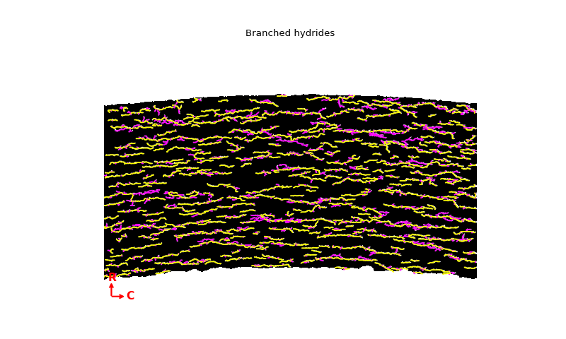
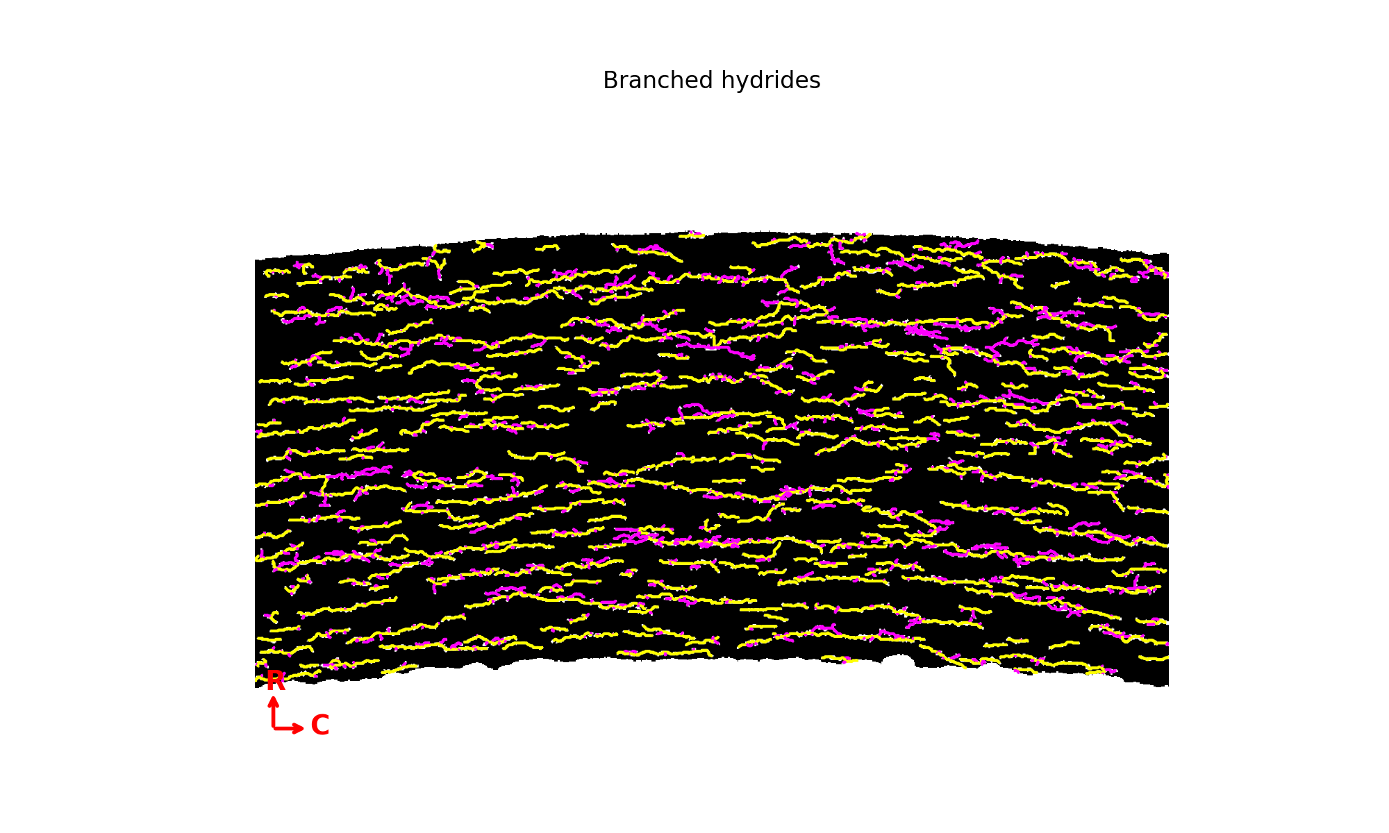
Branch Length Fraction

Here we want to determine the extent of branching within the microstrucutre, this is done in two ways: - In image form where the branches are coloured differently to the main hydride - BLF the length fraction of branches with respect to the toatal length of all hydrides in the microstrucutre

>>> # Calculate the branch length fraction
>>> skel,is_main,BLF = branch.branch_classification(thres);
>>>
>>>
>>> # Plot branching image
>>> fig, ax = plt.subplots(figsize=(10,6))
>>> ax = draw.overlay_skeleton_2d_class(
...     skel,
...     skeleton_color_source=lambda s: is_main,
...     skeleton_colormap='spring',
...     axes=ax
...      )
...
>>> plt.axis('off')
>>> plt.title('Branched hydrides')
>>> #plt_f.addScaleBar(ax[0], scale=scale, location=location)
>>> plt_f.addArrows(ax[0])
>>>
>>> print('The BLF is: {0:.4f}'.format(BLF))

(png, hires.png, pdf)

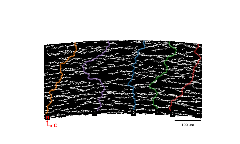
Crack Path

Here we want to determine potential crack paths through the microstrucutre, we input the thresholded image thres. After running once, the area around that path (radius set with kernel_size) is discounted, then the process is repeated num_runs times. Here the distance_weight makes moving in the circumferential direction more costly, note when comparing different micrographs, ensure that this parameter it is kept constant. We reccomend a weighting of 1.5 and a kernel size of 20.

>>> # Determing potential crack paths
>>> edist, path_list, cost_list = cp.det_crack_path(thres, crop_threshold, num_runs=5, kernel_size=20,distance_weight=1.5)

>>> # Plot possible crack paths
>>> fig, ax = plt.subplots(figsize=(10,6))
>>> list_costs = []
>>>
>>> for n, (p, c) in enumerate(zip(path_list, cost_list)):
...
...     im = ax.imshow(thres, cmap='gray')
...
...     #if n==0:
...       #  plt.colorbar(im,fraction=0.03, pad=0.01)
...     ax.scatter(p[:,1], p[:,0], s=10, alpha=0.1)
...     ax.text(p[-1][1], p[-1][0], s=str(n), c='w', bbox=dict(facecolor='black', edgecolor='black'))
...     plt.axis('off')
...     print('Run #{0}\tCost = {1:.2f}'.format(n,c))
...     list_costs.append(c)
...
>>> plt_f.addScaleBar(ax, scale=scale, location=location)
>>> plt_f.addArrows(ax)

(png, hires.png, pdf)

>>> # Histograms for plotting the costs of each path
>>> plt.hist(list_costs, bins=5, cumulative = True, color = "cornflowerblue", ec="cornflowerblue", label = "Cumulative Distribution Function")
>>> plt.hist(list_costs, bins=5, color = "lightpink", ec="lightpink", label = "Normal Histogram")
>>> plt.legend()
>>> plt.xlabel('Cost', fontsize="12")
>>> plt.ylabel('Frequency',fontsize="12")
>>> plt.title('Paths of Lowest Cost', fontweight="bold", fontsize="15")
>>> plt.show()

(png, hires.png, pdf)

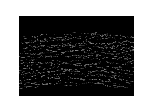
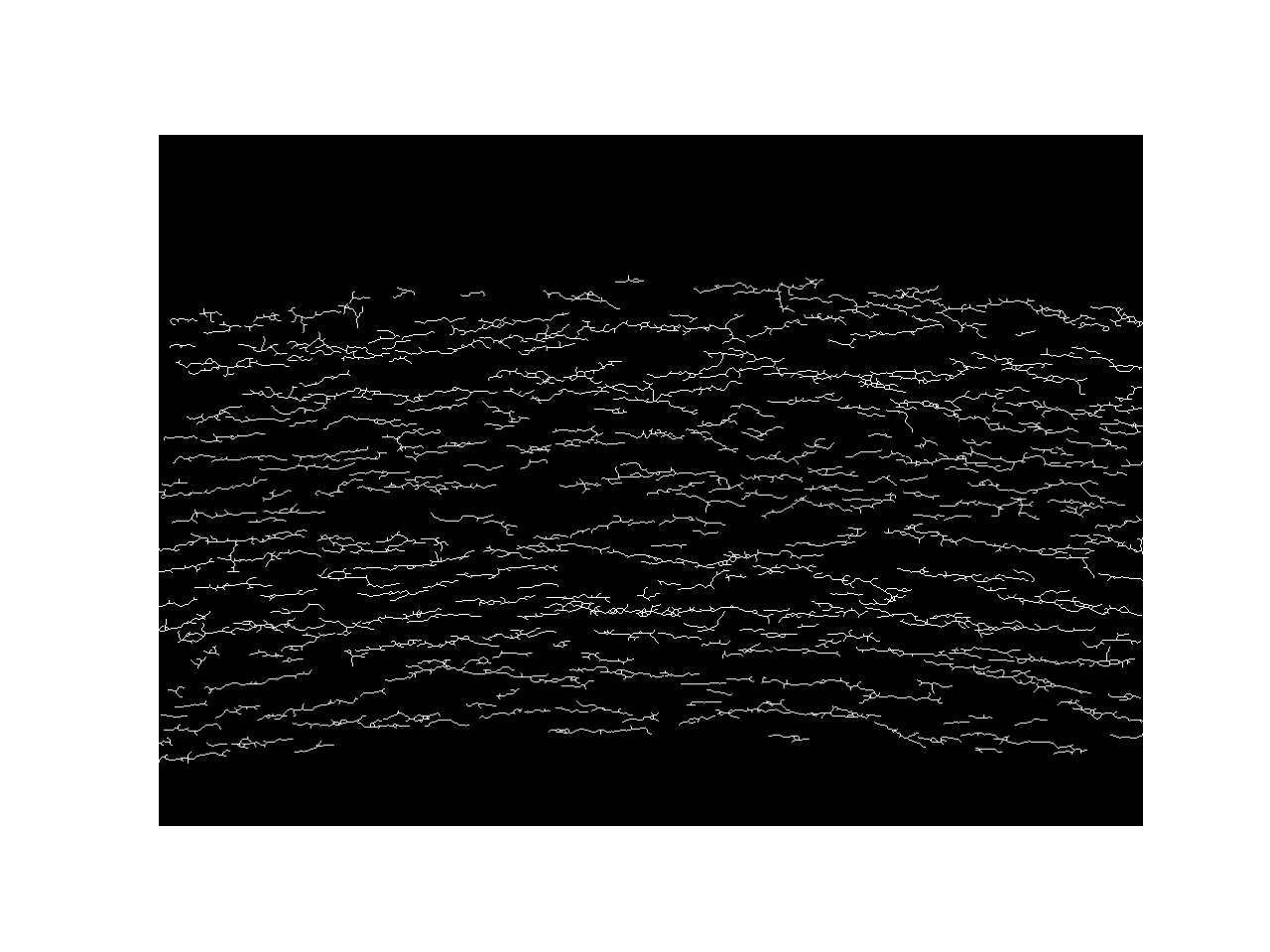
You can chose to skeletonize the image if you want, not reccomended unless there are too many hydrides to be able to distinguish between them.

>>> from skimage.morphology import skeletonize
>>> skeletonised = skeletonize(thres)
>>> plt.imshow(skeletonised,cmap='gray')
>>> plt.axis('off')
>>>
>>>
>>>

(png, hires.png, pdf)